System of equations. Detailed theory with examples (2020). Examples of systems of linear equations: solution method Writing a general solution of homogeneous and inhomogeneous linear algebraic systems using vectors of the fundamental system of solutions

Solving systems of linear algebraic equations (SLAE) is undoubtedly the most important topic of the linear algebra course. A huge number of problems from all branches of mathematics are reduced to solving systems of linear equations. These factors explain the reason for creating this article. The material of the article is selected and structured so that with its help you can

choose the optimal method for solving your system of linear algebraic equations,
study the theory of the chosen method,
solve your system of linear equations, having considered in detail the solutions of typical examples and problems.

Brief description of the material of the article.

First, we give all the necessary definitions, concepts, and introduce some notation.

Next, we consider methods for solving systems of linear algebraic equations in which the number of equations is equal to the number of unknown variables and which have a unique solution. First, let's focus on the Cramer method, secondly, we will show the matrix method for solving such systems of equations, and thirdly, we will analyze the Gauss method (the method of successive elimination of unknown variables). To consolidate the theory, we will definitely solve several SLAEs in various ways.

After that, we proceed to solving systems of linear algebraic equations of a general form, in which the number of equations does not coincide with the number of unknown variables or the main matrix of the system is degenerate. Let us formulate the Kronecker - Capelli theorem, which allows us to establish the compatibility of SLAE. Let us analyze the solution of systems (in the case of their compatibility) using the concept of the basis minor of a matrix. We will also consider the Gauss method and describe in detail the solutions of the examples.

Be sure to dwell on the structure of the general solution of homogeneous and inhomogeneous systems of linear algebraic equations. Let us give the concept of a fundamental system of solutions and show how the general solution of the SLAE is written using the vectors of the fundamental system of solutions. For a better understanding, let's look at a few examples.

In conclusion, we consider systems of equations that are reduced to linear ones, as well as various problems, in the solution of which SLAEs arise.

Page navigation.

Definitions, concepts, designations.

We will consider systems of p linear algebraic equations with n unknown variables (p may be equal to n ) of the form

Unknown variables, - coefficients (some real or complex numbers), - free members (also real or complex numbers).

This form of SLAE is called coordinate.

IN matrix form this system of equations has the form ,
Where - the main matrix of the system, - the matrix-column of unknown variables, - the matrix-column of free members.

If we add to the matrix A as the (n + 1)-th column the matrix-column of free terms, then we get the so-called expanded matrix systems of linear equations. Usually, the augmented matrix is denoted by the letter T, and the column of free members is separated by a vertical line from the rest of the columns, that is,

By solving a system of linear algebraic equations called a set of values of unknown variables , which turns all the equations of the system into identities. The matrix equation for the given values of the unknown variables also turns into an identity.

If a system of equations has at least one solution, then it is called joint.

If the system of equations has no solutions, then it is called incompatible.

If a SLAE has a unique solution, then it is called certain; if there is more than one solution, then - uncertain.

If the free terms of all equations of the system are equal to zero , then the system is called homogeneous, otherwise - heterogeneous.

Solution of elementary systems of linear algebraic equations.

If the number of system equations is equal to the number of unknown variables and the determinant of its main matrix is not equal to zero, then we will call such SLAEs elementary. Such systems of equations have a unique solution, and in the case of a homogeneous system, all unknown variables are equal to zero.

We started studying such SLAE in high school. When solving them, we took one equation, expressed one unknown variable in terms of others and substituted it into the remaining equations, then took the next equation, expressed the next unknown variable and substituted it into other equations, and so on. Or they used the addition method, that is, they added two or more equations to eliminate some unknown variables. We will not dwell on these methods in detail, since they are essentially modifications of the Gauss method.

The main methods for solving elementary systems of linear equations are the Cramer method, the matrix method and the Gauss method. Let's sort them out.

Solving systems of linear equations by Cramer's method.

Let us need to solve a system of linear algebraic equations

in which the number of equations is equal to the number of unknown variables and the determinant of the main matrix of the system is different from zero, that is, .

Let be the determinant of the main matrix of the system, and are determinants of matrices that are obtained from A by replacing 1st, 2nd, …, nth column respectively to the column of free members:

With such notation, the unknown variables are calculated by the formulas of Cramer's method as . This is how the solution of a system of linear algebraic equations is found by the Cramer method.

Example.

Cramer method .

Solution.

The main matrix of the system has the form . Calculate its determinant (if necessary, see the article):

Since the determinant of the main matrix of the system is different from zero, the system has a unique solution that can be found by Cramer's method.

Compose and calculate the necessary determinants (the determinant is obtained by replacing the first column in matrix A with a column of free members, the determinant - by replacing the second column with a column of free members, - by replacing the third column of matrix A with a column of free members):

Finding unknown variables using formulas :

Answer:

The main disadvantage of Cramer's method (if it can be called a disadvantage) is the complexity of calculating the determinants when the number of system equations is more than three.

Solving systems of linear algebraic equations by the matrix method (using the inverse matrix).

Let the system of linear algebraic equations be given in matrix form , where the matrix A has dimension n by n and its determinant is nonzero.

Since , then the matrix A is invertible, that is, there is an inverse matrix . If we multiply both parts of the equality by on the left, then we get a formula for finding the column matrix of unknown variables. So we got the solution of the system of linear algebraic equations by the matrix method.

Example.

Solve System of Linear Equations matrix method.

Solution.

We rewrite the system of equations in matrix form:

Because

then SLAE can be solved by the matrix method. Using the inverse matrix, the solution to this system can be found as .

Let's build an inverse matrix using a matrix of algebraic complements of the elements of matrix A (if necessary, see the article):

It remains to calculate - the matrix of unknown variables by multiplying the inverse matrix on the matrix-column of free members (if necessary, see the article):

Answer:

or in another notation x 1 = 4, x 2 = 0, x 3 = -1.

The main problem in finding solutions to systems of linear algebraic equations by the matrix method is the complexity of finding the inverse matrix, especially for square matrices of order higher than the third.

Solving systems of linear equations by the Gauss method.

Suppose we need to find a solution to a system of n linear equations with n unknown variables
the determinant of the main matrix of which is different from zero.

The essence of the Gauss method consists in the successive exclusion of unknown variables: first, x 1 is excluded from all equations of the system, starting from the second, then x 2 is excluded from all equations, starting from the third, and so on, until only the unknown variable x n remains in the last equation. Such a process of transforming the equations of the system for the successive elimination of unknown variables is called direct Gauss method. After the completion of the forward run of the Gaussian method, x n is found from the last equation, x n-1 is calculated from the penultimate equation using this value, and so on, x 1 is found from the first equation. The process of calculating unknown variables when moving from the last equation of the system to the first is called reverse Gauss method.

Let us briefly describe the algorithm for eliminating unknown variables.

We will assume that , since we can always achieve this by rearranging the equations of the system. We exclude the unknown variable x 1 from all equations of the system, starting from the second one. To do this, add the first equation multiplied by to the second equation of the system, add the first multiplied by to the third equation, and so on, add the first multiplied by to the nth equation. The system of equations after such transformations will take the form

where , a .

We would come to the same result if we expressed x 1 in terms of other unknown variables in the first equation of the system and substituted the resulting expression into all other equations. Thus, the variable x 1 is excluded from all equations, starting from the second.

Next, we act similarly, but only with a part of the resulting system, which is marked in the figure

To do this, add the second multiplied by to the third equation of the system, add the second multiplied by to the fourth equation, and so on, add the second multiplied by to the nth equation. The system of equations after such transformations will take the form

where , a . Thus, the variable x 2 is excluded from all equations, starting from the third.

Next, we proceed to the elimination of the unknown x 3, while acting similarly with the part of the system marked in the figure

So we continue the direct course of the Gauss method until the system takes the form

From this moment, we begin the reverse course of the Gauss method: we calculate x n from the last equation as , using the obtained value x n we find x n-1 from the penultimate equation, and so on, we find x 1 from the first equation.

Example.

Solve System of Linear Equations Gaussian method.

Solution.

Let's exclude the unknown variable x 1 from the second and third equations of the system. To do this, to both parts of the second and third equations, we add the corresponding parts of the first equation, multiplied by and by, respectively:

Now we exclude x 2 from the third equation by adding to its left and right parts the left and right parts of the second equation, multiplied by:

On this, the forward course of the Gauss method is completed, we begin the reverse course.

From the last equation of the resulting system of equations, we find x 3:

From the second equation we get .

From the first equation we find the remaining unknown variable and this completes the reverse course of the Gauss method.

Answer:

X 1 \u003d 4, x 2 \u003d 0, x 3 \u003d -1.

Solving systems of linear algebraic equations of general form.

In the general case, the number of equations of the system p does not coincide with the number of unknown variables n:

Such SLAEs may have no solutions, have a single solution, or have infinitely many solutions. This statement also applies to systems of equations whose main matrix is square and degenerate.

Kronecker-Capelli theorem.

Before finding a solution to a system of linear equations, it is necessary to establish its compatibility. The answer to the question when SLAE is compatible, and when it is incompatible, gives Kronecker–Capelli theorem:
for a system of p equations with n unknowns (p can be equal to n ) to be compatible it is necessary and sufficient that the rank of the main matrix of the system is equal to the rank of the extended matrix, that is, Rank(A)=Rank(T) .

Let us consider the application of the Kronecker-Cappelli theorem for determining the compatibility of a system of linear equations as an example.

Example.

Find out if the system of linear equations has solutions.

Solution.

. Let us use the method of bordering minors. Minor of the second order different from zero. Let's go over the third-order minors surrounding it:

Since all bordering third-order minors are equal to zero, the rank of the main matrix is two.

In turn, the rank of the augmented matrix is equal to three, since the minor of the third order

different from zero.

Thus, Rang(A) , therefore, according to the Kronecker-Capelli theorem, we can conclude that the original system of linear equations is inconsistent.

Answer:

There is no solution system.

So, we have learned to establish the inconsistency of the system using the Kronecker-Capelli theorem.

But how to find the solution of the SLAE if its compatibility is established?

To do this, we need the concept of the basis minor of a matrix and the theorem on the rank of a matrix.

The highest order minor of the matrix A, other than zero, is called basic.

It follows from the definition of the basis minor that its order is equal to the rank of the matrix. For a non-zero matrix A, there can be several basic minors; there is always one basic minor.

For example, consider the matrix .

All third-order minors of this matrix are equal to zero, since the elements of the third row of this matrix are the sum of the corresponding elements of the first and second rows.

The following minors of the second order are basic, since they are nonzero

Minors are not basic, since they are equal to zero.

Matrix rank theorem.

If the rank of a matrix of order p by n is r, then all elements of the rows (and columns) of the matrix that do not form the chosen basis minor are linearly expressed in terms of the corresponding elements of the rows (and columns) that form the basis minor.

What does the matrix rank theorem give us?

If, by the Kronecker-Capelli theorem, we have established the compatibility of the system, then we choose any basic minor of the main matrix of the system (its order is equal to r), and exclude from the system all equations that do not form the chosen basic minor. The SLAE obtained in this way will be equivalent to the original one, since the discarded equations are still redundant (according to the matrix rank theorem, they are a linear combination of the remaining equations).

As a result, after discarding the excessive equations of the system, two cases are possible.

If the number of equations r in the resulting system is equal to the number of unknown variables, then it will be definite and the only solution can be found by the Cramer method, the matrix method or the Gauss method.

Example.

Solution.

Rank of the main matrix of the system is equal to two, since the minor of the second order different from zero. Extended matrix rank is also equal to two, since the only minor of the third order is equal to zero

and the minor of the second order considered above is different from zero. Based on the Kronecker-Capelli theorem, one can assert the compatibility of the original system of linear equations, since Rank(A)=Rank(T)=2 .

As a basis minor, we take . It is formed by the coefficients of the first and second equations:

The third equation of the system does not participate in the formation of the basic minor, so we exclude it from the system based on the matrix rank theorem:

Thus we have obtained an elementary system of linear algebraic equations. Let's solve it by Cramer's method:

Answer:

x 1 \u003d 1, x 2 \u003d 2.

If the number of equations r in the resulting SLAE is less than the number of unknown variables n, then we leave the terms that form the basic minor in the left parts of the equations, and transfer the remaining terms to the right parts of the equations of the system with the opposite sign.

The unknown variables (there are r of them) remaining on the left-hand sides of the equations are called main.

Unknown variables (there are n - r of them) that ended up on the right side are called free.

Now we assume that the free unknown variables can take arbitrary values, while the r main unknown variables will be expressed in terms of the free unknown variables in a unique way. Their expression can be found by solving the resulting SLAE by the Cramer method, the matrix method, or the Gauss method.

Let's take an example.

Example.

Solve System of Linear Algebraic Equations .

Solution.

Find the rank of the main matrix of the system by the bordering minors method. Let us take a 1 1 = 1 as a non-zero first-order minor. Let's start searching for a non-zero second-order minor surrounding this minor:

So we found a non-zero minor of the second order. Let's start searching for a non-zero bordering minor of the third order:

Thus, the rank of the main matrix is three. The rank of the augmented matrix is also equal to three, that is, the system is consistent.

The found non-zero minor of the third order will be taken as the basic one.

For clarity, we show the elements that form the basis minor:

We leave the terms participating in the basic minor on the left side of the equations of the system, and transfer the rest with opposite signs to the right sides:

We give free unknown variables x 2 and x 5 arbitrary values, that is, we take , where are arbitrary numbers. In this case, the SLAE takes the form

We solve the obtained elementary system of linear algebraic equations by the Cramer method:

Hence, .

In the answer, do not forget to indicate free unknown variables.

Answer:

Where are arbitrary numbers.

Summarize.

To solve a system of linear algebraic equations of a general form, we first find out its compatibility using the Kronecker-Capelli theorem. If the rank of the main matrix is not equal to the rank of the extended matrix, then we conclude that the system is inconsistent.

If the rank of the main matrix is equal to the rank of the extended matrix, then we choose the basic minor and discard the equations of the system that do not participate in the formation of the chosen basic minor.

If the order of the basis minor is equal to the number of unknown variables, then the SLAE has a unique solution, which can be found by any method known to us.

If the order of the basis minor is less than the number of unknown variables, then we leave the terms with the main unknown variables on the left side of the equations of the system, transfer the remaining terms to the right sides and assign arbitrary values to the free unknown variables. From the resulting system of linear equations, we find the main unknown variables by the Cramer method, the matrix method or the Gauss method.

Gauss method for solving systems of linear algebraic equations of general form.

Using the Gauss method, one can solve systems of linear algebraic equations of any kind without their preliminary investigation for compatibility. The process of successive elimination of unknown variables makes it possible to draw a conclusion about both the compatibility and inconsistency of the SLAE, and if a solution exists, it makes it possible to find it.

From the point of view of computational work, the Gaussian method is preferable.

See its detailed description and analyzed examples in the article Gauss method for solving systems of linear algebraic equations of general form.

Recording the general solution of homogeneous and inhomogeneous linear algebraic systems using the vectors of the fundamental system of solutions.

In this section, we will focus on joint homogeneous and inhomogeneous systems of linear algebraic equations that have an infinite number of solutions.

Let's deal with homogeneous systems first.

Fundamental decision system A homogeneous system of p linear algebraic equations with n unknown variables is a set of (n – r) linearly independent solutions of this system, where r is the order of the basis minor of the main matrix of the system.

If we designate linearly independent solutions of a homogeneous SLAE as X (1) , X (2) , …, X (n-r) (X (1) , X (2) , …, X (n-r) are matrices columns of dimension n by 1 ) , then the general solution of this homogeneous system is represented as a linear combination of vectors of the fundamental system of solutions with arbitrary constant coefficients С 1 , С 2 , …, С (n-r), that is, .

What does the term general solution of a homogeneous system of linear algebraic equations (oroslau) mean?

The meaning is simple: the formula specifies all possible solutions to the original SLAE, in other words, taking any set of values of arbitrary constants C 1 , C 2 , ..., C (n-r) , according to the formula we will get one of the solutions of the original homogeneous SLAE.

Thus, if we find a fundamental system of solutions, then we can set all solutions of this homogeneous SLAE as .

Let us show the process of constructing a fundamental system of solutions for a homogeneous SLAE.

We choose the basic minor of the original system of linear equations, exclude all other equations from the system, and transfer to the right-hand side of the equations of the system with opposite signs all terms containing free unknown variables. Let's give the free unknown variables the values 1,0,0,…,0 and calculate the main unknowns by solving the resulting elementary system of linear equations in any way, for example, by the Cramer method. Thus, X (1) will be obtained - the first solution of the fundamental system. If we give the free unknowns the values 0,1,0,0,…,0 and calculate the main unknowns, then we get X (2) . And so on. If we give the free unknown variables the values 0,0,…,0,1 and calculate the main unknowns, then we get X (n-r) . This is how the fundamental system of solutions of the homogeneous SLAE will be constructed and its general solution can be written in the form .

For inhomogeneous systems of linear algebraic equations, the general solution is represented as

Let's look at examples.

Example.

Find the fundamental system of solutions and the general solution of a homogeneous system of linear algebraic equations .

Solution.

The rank of the main matrix of homogeneous systems of linear equations is always equal to the rank of the extended matrix. Let us find the rank of the main matrix by the method of fringing minors. As a nonzero minor of the first order, we take the element a 1 1 = 9 of the main matrix of the system. Find the bordering non-zero minor of the second order:

A minor of the second order, different from zero, is found. Let's go through the third-order minors bordering it in search of a non-zero one:

All bordering minors of the third order are equal to zero, therefore, the rank of the main and extended matrix is two. Let's take the basic minor. For clarity, we note the elements of the system that form it:

The third equation of the original SLAE does not participate in the formation of the basic minor, therefore, it can be excluded:

We leave the terms containing the main unknowns on the right-hand sides of the equations, and transfer the terms with free unknowns to the right-hand sides:

Let us construct a fundamental system of solutions to the original homogeneous system of linear equations. The fundamental system of solutions of this SLAE consists of two solutions, since the original SLAE contains four unknown variables, and the order of its basic minor is two. To find X (1), we give the free unknown variables the values x 2 \u003d 1, x 4 \u003d 0, then we find the main unknowns from the system of equations
.

Systems m linear equations with n unknown.
Solving a system of linear equations is such a set of numbers ( x 1 , x 2 , …, x n), substituting which into each of the equations of the system, the correct equality is obtained.
Where a ij , i = 1, …, m; j = 1, …, n are the coefficients of the system;
b i , i = 1, …, m- free members;
x j , j = 1, …, n- unknown.
The above system can be written in matrix form: A X = B,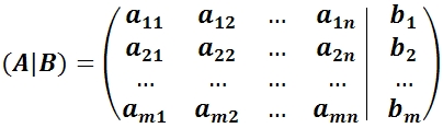

Where ( A|B) is the main matrix of the system;
A— extended matrix of the system;
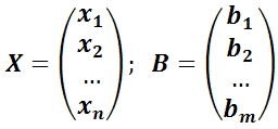
X— column of unknowns;
B is a column of free members.
If the matrix B is not a null matrix ∅, then this system of linear equations is called inhomogeneous.
If the matrix B= ∅, then this system of linear equations is called homogeneous. A homogeneous system always has a zero (trivial) solution: x 1 \u003d x 2 \u003d ..., x n \u003d 0.
Joint system of linear equations is a system of linear equations that has a solution.
Inconsistent system of linear equations is a system of linear equations that has no solution.
Certain system of linear equations is a system of linear equations that has a unique solution.
Indefinite system of linear equations is a system of linear equations that has an infinite number of solutions.
Systems of n linear equations with n unknowns
If the number of unknowns is equal to the number of equations, then the matrix is square. The matrix determinant is called the main determinant of the system of linear equations and is denoted by the symbol Δ.
Cramer method for solving systems n linear equations with n unknown.
Cramer's rule.
If the main determinant of a system of linear equations is not equal to zero, then the system is consistent and defined, and the only solution is calculated using the Cramer formulas:
where Δ i are the determinants obtained from the main determinant of the system Δ by replacing i th column to the column of free members. .
Systems of m linear equations with n unknowns
Kronecker-Cappelli theorem.

For this system of linear equations to be consistent, it is necessary and sufficient that the rank of the matrix of the system be equal to the rank of the extended matrix of the system, rank(Α) = rank(Α|B).
If rang(Α) ≠ rang(Α|B), then the system obviously has no solutions.
If rank(Α) = rank(Α|B), then two cases are possible:
1) rang(Α) = n(to the number of unknowns) - the solution is unique and can be obtained by Cramer's formulas;
2) rank(Α)< n − there are infinitely many solutions.
Gauss method for solving systems of linear equations

Let's compose the augmented matrix ( A|B) of the given system of coefficients at the unknown and right-hand sides.
The Gaussian method or the elimination of unknowns method consists in reducing the augmented matrix ( A|B) with the help of elementary transformations over its rows to a diagonal form (to an upper triangular form). Returning to the system of equations, all unknowns are determined.
Elementary transformations on strings include the following:
1) swapping two lines;
2) multiplying a string by a number other than 0;
3) adding to the string another string multiplied by an arbitrary number;
4) discarding a null string.
An extended matrix reduced to a diagonal form corresponds to a linear system equivalent to the given one, the solution of which does not cause difficulties. .
System of homogeneous linear equations.
The homogeneous system has the form:

it corresponds to the matrix equation A X = 0.
1) A homogeneous system is always consistent, since r(A) = r(A|B), there is always a zero solution (0, 0, …, 0).
2) For a homogeneous system to have a nonzero solution, it is necessary and sufficient that r = r(A)< n , which is equivalent to Δ = 0.
3) If r< n , then Δ = 0, then there are free unknowns c 1 , c 2 , …, c n-r, the system has nontrivial solutions, and there are infinitely many of them.
4) General solution X at r< n can be written in matrix form as follows:
X \u003d c 1 X 1 + c 2 X 2 + ... + c n-r X n-r,
where are the solutions X 1 , X 2 , …, X n-r form a fundamental system of solutions.
5) The fundamental system of solutions can be obtained from the general solution of the homogeneous system:

,
if we sequentially assume the values of the parameters to be (1, 0, …, 0), (0, 1, …, 0), …, (0, 0, …, 1).
Decomposition of the general solution in terms of the fundamental system of solutions is a record of the general solution as a linear combination of solutions belonging to the fundamental system.
Theorem. For a system of linear homogeneous equations to have a nonzero solution, it is necessary and sufficient that Δ ≠ 0.
So, if the determinant is Δ ≠ 0, then the system has a unique solution.
If Δ ≠ 0, then the system of linear homogeneous equations has an infinite number of solutions.
Theorem. For a homogeneous system to have a nonzero solution, it is necessary and sufficient that r(A)< n .
Proof:
1) r can't be more n(matrix rank does not exceed the number of columns or rows);
2) r< n , because If r=n, then the main determinant of the system Δ ≠ 0, and, according to Cramer's formulas, there is a unique trivial solution x 1 \u003d x 2 \u003d ... \u003d x n \u003d 0, which contradicts the condition. Means, r(A)< n .
Consequence. In order for a homogeneous system n linear equations with n unknowns has a nonzero solution, it is necessary and sufficient that Δ = 0.

Systems of linear equations. Lecture 6

Systems of linear equations.

Basic concepts.

view system

called system - linear equations with unknowns.

Numbers , , are called system coefficients.

Numbers are called free members of the system, – system variables. Matrix

called the main matrix of the system, and the matrix

– expanded matrix system. Matrices - columns

And correspondingly matrices of free members and unknowns of the system. Then, in matrix form, the system of equations can be written as . System solution is called the values of the variables, when substituting which, all the equations of the system turn into true numerical equalities. Any solution of the system can be represented as a matrix-column. Then the matrix equality is true.

The system of equations is called joint if it has at least one solution and incompatible if it has no solution.

To solve a system of linear equations means to find out whether it is compatible and, if it is compatible, to find its general solution.

The system is called homogeneous if all its free terms are equal to zero. A homogeneous system is always compatible because it has a solution

The Kronecker-Kopelli theorem.

The answer to the question of the existence of solutions of linear systems and their uniqueness allows us to obtain the following result, which can be formulated as the following statements about a system of linear equations with unknowns

(1)

Theorem 2. The system of linear equations (1) is consistent if and only if the rank of the main matrix is equal to the rank of the extended one (.

Theorem 3. If the rank of the main matrix of a joint system of linear equations is equal to the number of unknowns, then the system has a unique solution.

Theorem 4. If the rank of the main matrix of a joint system is less than the number of unknowns, then the system has an infinite number of solutions.

Rules for solving systems.

3. Find the expression of the main variables in terms of the free ones and get the general solution of the system.

4. By giving arbitrary values to free variables, all values of the main variables are obtained.

Methods for solving systems of linear equations.

Inverse matrix method.

and , i.e., the system has a unique solution. We write the system in matrix form

Where , , .

Multiply both sides of the matrix equation on the left by the matrix

Since , we obtain , from which we obtain equality for finding unknowns

Example 27. Using the inverse matrix method, solve the system of linear equations

Solution. Denote by the main matrix of the system

Let , then we find the solution by the formula .

Let's calculate .

Since , then the system has a unique solution. Find all algebraic additions

, ,

Thus

Let's check

The inverse matrix is found correctly. From here, using the formula , we find the matrix of variables .

Comparing the values of the matrices, we get the answer: .

Cramer's method.

Let a system of linear equations with unknowns be given

and , i.e., the system has a unique solution. We write the solution of the system in matrix form or

Denote

. . . . . . . . . . . . . . ,

Thus, we obtain formulas for finding the values of the unknowns, which are called Cramer's formulas.

Example 28. Solve the following system of linear equations using Cramer's method .

Solution. Find the determinant of the main matrix of the system

Since , then , the system has a unique solution.

Find the remaining determinants for Cramer's formulas

Using Cramer's formulas, we find the values of the variables

Gauss method.

The method consists in sequential exclusion of variables.

Let a system of linear equations with unknowns be given.

The Gaussian solution process consists of two steps:

At the first stage, the extended matrix of the system is reduced to the stepwise form with the help of elementary transformations

where , which corresponds to the system

After that the variables are considered free and in each equation are transferred to the right side.

At the second stage, the variable is expressed from the last equation, the resulting value is substituted into the equation. From this equation

variable is expressed. This process continues until the first equation. The result is an expression of the principal variables in terms of the free variables .

Example 29. Solve the following system using the Gaussian method

Solution. Let us write out the extended matrix of the system and reduce it to the step form

Because is greater than the number of unknowns, then the system is compatible and has an infinite number of solutions. Let us write down the system for the step matrix

The determinant of the extended matrix of this system, composed of the first three columns, is not equal to zero, so we consider it to be basic. Variables

Will be basic and the variable will be free. Let's move it in all equations to the left side

From the last equation we express

Substituting this value into the penultimate second equation, we get

where . Substituting the values of the variables and into the first equation, we find . We write the answer in the following form

WITH n unknown is a system of the form:

Where aij And b i (i=1,…,m; b=1,…,n) are some known numbers, and x 1 ,…,x n- unknown numbers. In the notation of the coefficients aij index i determines the number of the equation, and the second j is the number of the unknown at which this coefficient is located.

Homogeneous system - when all free members of the system are equal to zero ( b 1 = b 2 = ... = b m = 0), the opposite situation is heterogeneous system.

Square system - when the number m equations equals the number n unknown.

System solution- set n numbers c 1 , c 2 , …, c n , such that the substitution of all c i instead of x i into a system turns all its equations into identities.

Joint system - when the system has at least one solution, and incompatible system when the system has no solutions.

A joint system of this kind (as given above, let it be (1)) can have one or more solutions.

Solutions c 1 (1) , c 2 (1) , …, c n (1) And c 1 (2) , c 2 (2) , …, c n (2) joint system of type (1) will various, when even 1 of the equalities is not satisfied:

c 1 (1) = c 1 (2) , c 2 (1) = c 2 (2) , …, c n (1) = c n (2) .

A joint system of type (1) will certain when it has only one solution; when a system has at least 2 different solutions, it becomes underdetermined. When there are more equations than unknowns, the system is redefined.

The coefficients for the unknowns are written as a matrix:

It is called system matrix.

The numbers that are on the right side of the equations, b 1 ,…,b m are free members.

Aggregate n numbers c 1 ,…,c n is a solution to this system when all equations of the system turn into equality after substituting numbers in them c 1 ,…,c n instead of the corresponding unknowns x 1 ,…,x n.

When solving a system of linear equations, 3 options may arise:

1. The system has only one solution.

2. The system has an infinite number of solutions. For example, . The solution of this system will be all pairs of numbers that differ in sign.

3. The system has no solutions. For example, , if a solution exists, then x 1 + x 2 equals 0 and 1 at the same time.

Methods for solving systems of linear equations.

Direct Methods give an algorithm by which the exact solution is found SLAU(systems of linear algebraic equations). And if the accuracy were absolute, they would have found it. A real electric computer, of course, works with an error, so the solution will be approximate.

Many practical problems are reduced to solving systems of algebraic equations of the 1st degree or, as they are usually called, systems of linear equations. We will learn to solve any such systems, without even requiring that the number of equations coincide with the number of unknowns.

In general, the system of linear equations is written as follows:

Here are the numbers aij– odds systems, b i – free members, x i- symbols unknown . It is very convenient to introduce matrix notation:- main matrix of the system, – matrix-column of free terms, – matrix-column of unknowns. Then the system can be written as follows: AX=B or, in more detail:

If, on the left side of this equality, perform matrix multiplication according to the usual rules and equate the elements of the resulting column to the elements IN, then we will arrive at the original system notation.

Example 14. We write the same system of linear equations in two different ways:

The system of linear equations is usually called joint , if it has at least one solution, and incompatible, if there are no solutions.

In our example, the system is compatible, the column is its solution:

This solution can also be written without matrices: x=2,y=1 . We will call the system of equations uncertain , if it has more than one solution, and certain if the solution is unique.

Example 15. The system is indeterminate. For example, are its solutions. The reader can find many other solutions to this system.

Let's learn how to solve systems of linear equations first in a particular case. The system of equations OH=IN we will call Kramerovskaya , if its main matrix A are square and non-degenerate. In other words, in the Cramerian system, the number of unknowns coincides with the number of equations and .

Theorem 6. (Cramer's rule). The Cramer system of linear equations has a unique solution given by the formulas:

where is the determinant of the main matrix, is the determinant obtained from D replacement i-th column with a column of free members.

Comment. Cramer systems can also be solved in another way, using the inverse matrix. We write such a system in matrix form: AX=IN. Since , then there is an inverse matrix A –1 . We multiply the matrix equality by A –1 left: A –1 OH=A –1 IN. Because A –1 OH=EX=X, then the solution of the system is found: X= A –1 IN.We will call this method of solution matrix . We emphasize once again that it is suitable only for Cramer systems - in other cases, the inverse matrix does not exist. The reader will find the analyzed examples of the application of the matrix method and the Cramer method below.

Let us finally study the general case, the system m linear equations with n unknown. To solve it, apply Gauss method , which we will consider in detail. For an arbitrary system of equations OH=IN write out extended matrix. So it is customary to call the matrix, which will turn out if the main matrix A on the right, add a column of free members IN:

As in the calculation of the rank, with the help of elementary transformations of rows and permutations of columns, we will bring our matrix to a trapezoidal shape. In this case, of course, the system of equations corresponding to the matrix will change, but will be is tantamount to original (ᴛ.ᴇ. will have the same solutions). Indeed, rearranging or adding equations will not change the solutions. Rearranging Columns - Too: Equations x 1+3x2+7x3=4 And x 1+7x3+3x2=4, are, of course, equivalent. It is only necessary to write down which unknown column corresponds to. We do not rearrange the column of free members - it is usually separated from others by a dotted line in the matrix. Zero rows appearing in the matrix can be omitted.

Example 1. Solve the system of equations:

Solution. We write out the extended matrix and bring it to a trapezoidal form. Sign ~ now will mean not only the coincidence of ranks, but also the equivalence of the corresponding systems of equations.

~ . Let's explain the steps taken.

Action 1. The 1st line was added to the 2nd line, multiplying it by (–2). To the 3rd and 4th lines they added the 1st, multiplying it by (–3). The purpose of these operations is to get zeros in the first column, below the main diagonal.

Action 2. Since on the diagonal place (2,2) there is 0 , I had to rearrange the 2nd and 3rd columns. To remember this permutation, we wrote the symbols of the unknowns on top.

Action 3. To the 3rd line they added the 2nd, multiplying it by (–2). The 2nd line was added to the 4th line. The goal is to get zeros in the second column, below the main diagonal.

Action 4. Zero lines can be removed.

So, the matrix is reduced to a trapezoidal shape. Her rank r=2 . Unknown x 1, x 3- basic; x 2, x 4- free. Let us assign arbitrary values to the free unknowns:

x 2= a, x 4= b.

Here a, b are any number. Now from the last equation of the new system

x 3+x4= –3

find x 3: x 3= –3 –b. Rising up, from the first equation

x 1+3x 3+2x 2+4x4= 5

find x 1: x 1=5 –3(–3 –b)–2a–4b= 14 –2a–b.

We write down the general solution:

x 1=14 –2a–b, x2=a,x3=–3 –b,x4=b.

You can write the general solution in the form of a matrix-column:

For specific values a And b, you can get private solutions. For example, when a=0,b=1 we obtain: is one of the solutions of the system.

Remarks. In the Gauss method algorithm, we have seen (case 1), that the inconsistency of the system of equations is connected with the mismatch of the ranks of the main and extended matrices. We present the following important theorem without proof.

Theorem 7 (Kronecker-Capelli). A system of linear equations is consistent if and only if the rank of the main matrix is equal to the rank of the extended matrix of the system.

Systems of linear equations - concept and types. Classification and features of the category "Systems of linear equations" 2017, 2018.

- SYSTEMS OF LINEAR EQUATIONS

So that its rows (or columns) are linearly dependent. Let a system containing m linear equations with n unknowns be given: 5.1. Let us introduce the following notation. 5.2., - the matrix of the system - its extended matrix. - column of free members. - column of unknowns. If... .

- P.1. Reduction of a system of linear equations to a problem

non-linear optimization (NNO) and vice versa. Statement of the ZNO problem: Find (8.1) a minimum or a maximum in some area D. As we remember from the mat. analysis, one should equate the partial derivatives to zero. Thus, ZNO (8.1) was reduced to SLE (8.2) (8.2) of n nonlinear equations. ... .

- Inhomogeneous systems of linear equations

Lecture 15 Consider an inhomogeneous system (16) If the corresponding coefficients of a homogeneous system (7) are equal to the corresponding coefficients of an inhomogeneous system (16), then the homogeneous system (7) is called the corresponding inhomogeneous system (16). Theorem. If... [read more] .

7.1 Homogeneous systems of linear equations. Let a homogeneous system of linear equations be given (*) Suppose that a set of numbers is some kind of solution to this system. Then the set of numbers is also a solution. This is verified by direct substitution into the equations of the system.... .

- The structure of the solution set of the system of linear equations

Table 3 Stages of motor development of a child Stage Age Indicators of motor development time of birth up to 4 months Formation of control over the position of the head and the possibility of its free orientation in space 4-6 months mastering the initial ... .

- Systems of linear equations (SLE). Solution of a system of linear equations. Elementary SLE transformations. Elementary matrix transformations.

Definition 1. A system of linear equations of the form (1) , where, the field, is called a system of m linear equations with n unknowns over the field, are the coefficients of the unknowns, are the free members of the system (1). Definition 2. An ordered n-ka (), where, is called the solution of a system of linear ... .